Discrete Diffusion for Molecular Generation with RL and Natural Language Steering
Designing drug-like molecules is, at its core, a search problem over an enormous discrete space. This post walks through how we built a modular architecture that learns the grammar of that space, then learned to steer it — first with reinforcement learning toward measurable chemical properties, then with natural language descriptions.
The problem with existing approaches
Traditional generative models for molecules have three recurring issues.
VAEs can only optimize in the continuous latent space, not directly in molecular space. GANs require expensive compute and suffer from mode collapse. Autoregressive models generate token by token left to right: if the model makes a mistake at position i, everything after it is already wrong — it either never closes the ring it opened, or closes it in the wrong place.
The validity problem is especially sharp. Standard SMILES notation encodes molecules as text strings, but most randomly sampled strings are chemically invalid: unclosed rings, violated valence rules, mismatched parentheses. Models have to learn chemistry syntax, and many fail.
Why SELFIES
We chose SELFIES (Self-Referencing Embedded Strings) as our molecular representation. Any SELFIES token sequence decodes to a valid molecule by construction. The grammar is designed so the decoder can always find a valid interpretation — even if the model guesses a ring count that exceeds what is chemically possible, SELFIES adjusts automatically.
This gives 100% chemical validity by construction, not by filtering or correction. Our closest comparison (TGM-DLM, 180M parameters) reaches only 87.1% validity even with a dedicated correction network as a second phase.
The tradeoff: SELFIES sequences are longer than SMILES, and ring closures use a count token that creates a dependency problem we return to in the failure analysis.
Architecture
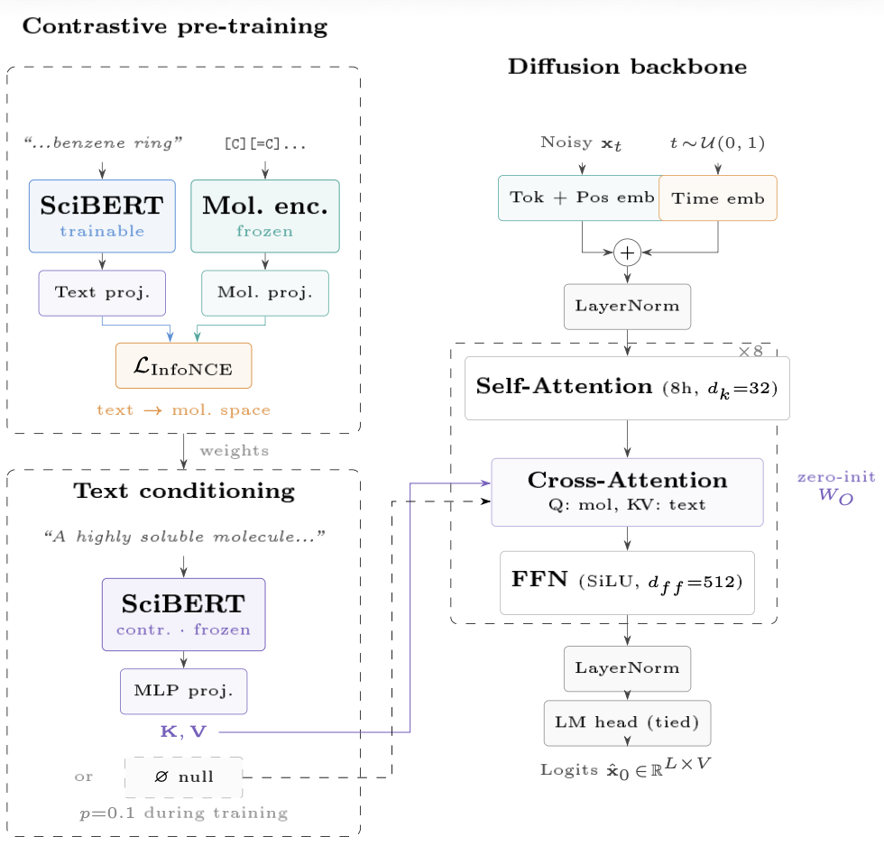
The architecture has three coupled components. The diffusion backbone is a bidirectional transformer that takes noisy token sequences $\mathbf{x}_t$ at timestep $t \sim \mathcal{U}(0,1)$ and predicts the clean $\hat{x}_0$ directly (rather than predicting noise, as in continuous diffusion). Each of the 8 transformer blocks applies self-attention over the full SELFIES sequence, then cross-attention where the molecule tokens form the queries and the text embedding provides keys and values. The cross-attention output projection $W_O$ is zero-initialized: at the start of text-conditioning fine-tuning, cross-attention contributes nothing, so the backbone behaves identically to the pretrained unconditional model. This lets us add text conditioning without retraining from scratch.
Contrastive pre-training (top-left) aligns the text and molecule embedding spaces before fine-tuning. SciBERT is trained while the molecule encoder stays frozen; both pass through learned projectors and are pulled together via InfoNCE loss. The result is a text encoder whose representation geometry matches chemical space — which matters because cross-attention uses these representations directly as keys and values.
Text conditioning (bottom-left) then uses the contrastively-trained SciBERT, now frozen, passed through an MLP projector to match the transformer’s hidden dimension. During training, text conditioning is dropped with probability 0.1 (null token ∅ substituted), enabling classifier-free guidance at inference.
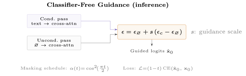
At inference, CFG runs two forward passes — one conditioned on the text prompt, one with the null token — and amplifies the difference by a guidance scale s:
\[\varepsilon = \varepsilon_\varnothing + s \cdot (\varepsilon_c - \varepsilon_\varnothing)\]The guided logits $\hat{x}_0$ are what the MaskGIT sampler uses for token selection. Setting $s = 0$ recovers the unconditional model; higher $s$ steers more aggressively toward the text description at the cost of diversity. The training loss is $\mathcal{L} = (1-t) \cdot \text{CE}(\hat{x}_0, x_0)$: the $(1-t)$ weighting upweights nearly-clean timesteps, where prediction errors matter most for final sample quality.
We built and tested three scales on the same architecture: 4.4M parameters (hidden 256, 8 layers, 8 heads) on a MacBook for RL experiments; 27M parameters (hidden 512) for text conditioning; and 150M on a GPU cluster for the scaling study. Only the hidden dimension changes between scales.
Training: MaskGIT-style discrete diffusion
Training follows the MaskGIT approach. For each batch, take a real SELFIES sequence, randomly mask a fraction of tokens using a cosine schedule $\alpha_t = \cos^2!\left(\tfrac{t\pi}{2}\right)$, then predict the original tokens at masked positions using standard cross-entropy. One forward pass per batch.
The cosine schedule means early in training, most tokens are visible (easy task); later, most are masked (hard task). We apply timestep weighting so that positions at low t (nearly clean sequences) receive higher loss weight — these are the most critical for final output fidelity.
Generation reverses this process over 50 iterative steps:
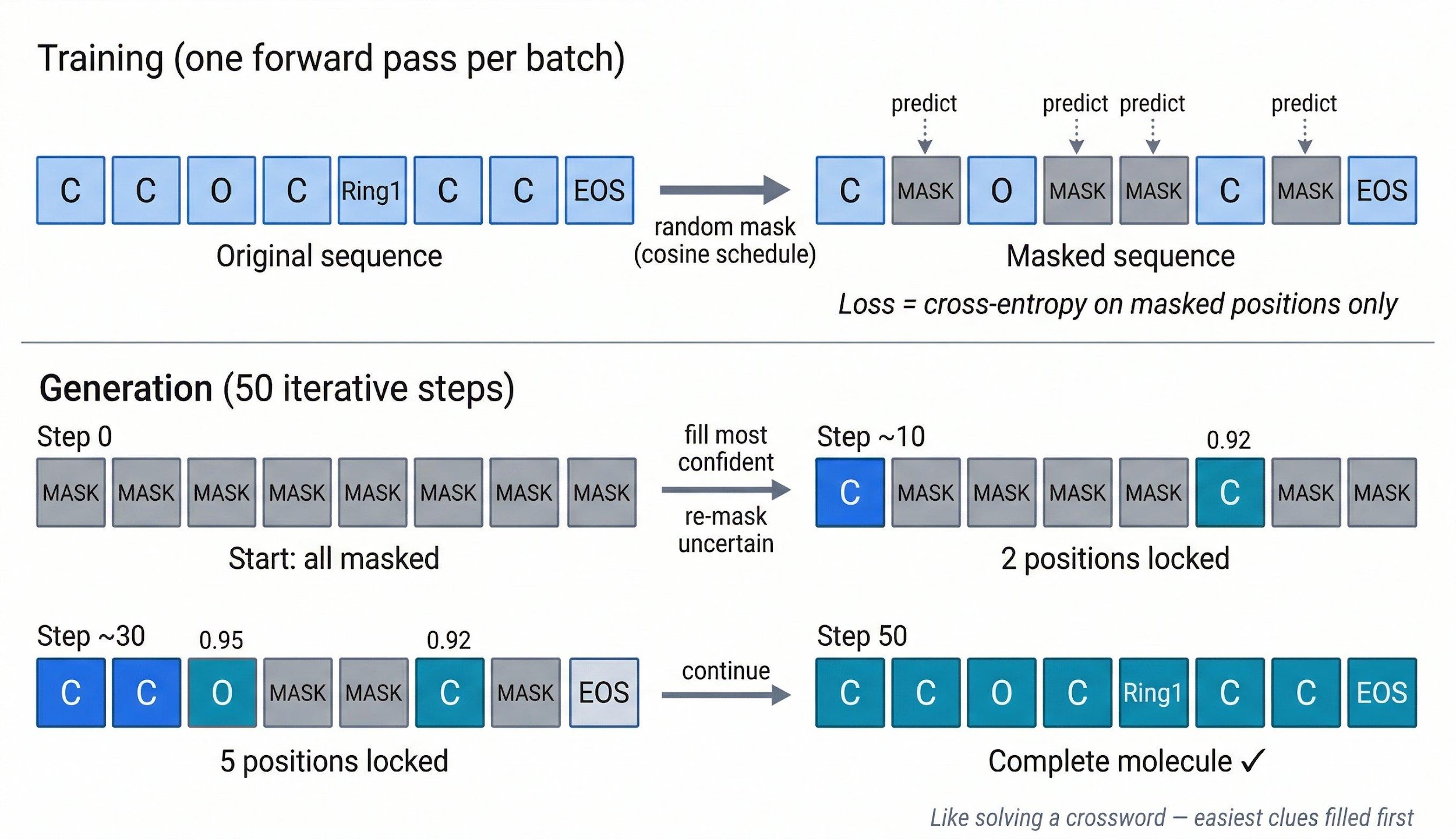
Start with all positions masked. At each step, predict all positions simultaneously, sample tokens, measure confidence (the softmax probability of the sampled token), lock the most confident positions, and re-mask the uncertain ones. Like solving a crossword puzzle: fill in the easiest clues first and use them as context for the harder ones.
Pretraining results on ZINC250K (500 generated molecules):
| Metric | Value |
|---|---|
| Validity | 100% |
| Uniqueness | 100% |
| Novelty | 100% |
| Diversity | 0.851 |
| Scaffold diversity | 954 / 1000 |
| Mean QED | 0.742 |
| QED KL vs ZINC250K | 0.022 |
| Lipinski pass rate | 99.4% |
100% novelty means zero overlap with the 249K training molecules — the model generalized rather than memorized. A QED KL of 0.022 means the generated distribution is statistically indistinguishable from the training distribution. But reproducing the distribution is not the same as controlling it. Mean QED of 0.742 is just the dataset average.
RL for property optimization: the per-step gradient problem
We used REINFORCE to optimize QED (a drug-likeness score from 0 to 1). The standard approach failed completely.
The naive recipe: generate a molecule, score it, compute the log probability of the sequence in a single forward pass at t=0, apply REINFORCE. This collapsed QED from 0.742 to 0.38.
The reason is not obvious until you think carefully about how MaskGIT generation works. In autoregressive language models, generation is the log probability computation — each forward pass generates the next token and produces its log probability. In MaskGIT, generation is 50 iterative steps with confidence-based token locking. A single forward pass at t=0 evaluates the model under conditions it never sees during generation. The gradient flows through the wrong path.
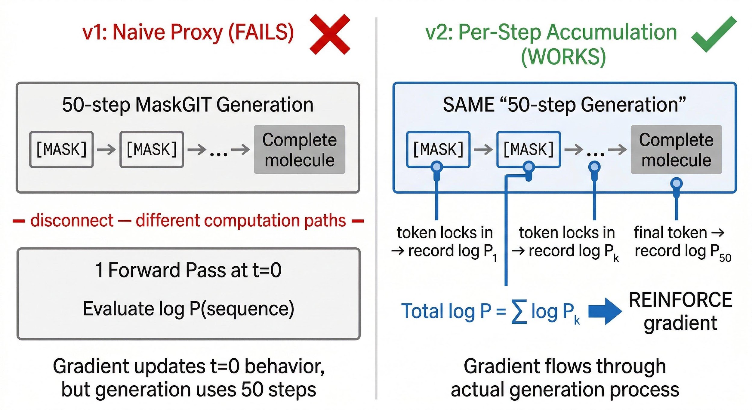
The fix: instrument the generation loop. At each denoising step, when a token transitions from masked to committed, record its log probability. Sum across all 50 steps:
\[\log P_\text{total} = \sum_k \log P_k\]The REINFORCE gradient now flows through the actual generation process. QED improved from 0.742 to 0.837.
This is the same principle as DDPO (Black et al., Berkeley 2023), which established per-step policy gradients for continuous diffusion in image generation. We arrived at it through debugging and found the connection afterward.
Reward shaping
With the gradient problem fixed, we ran four configurations in sequence, each motivated by what we measured in the previous result:
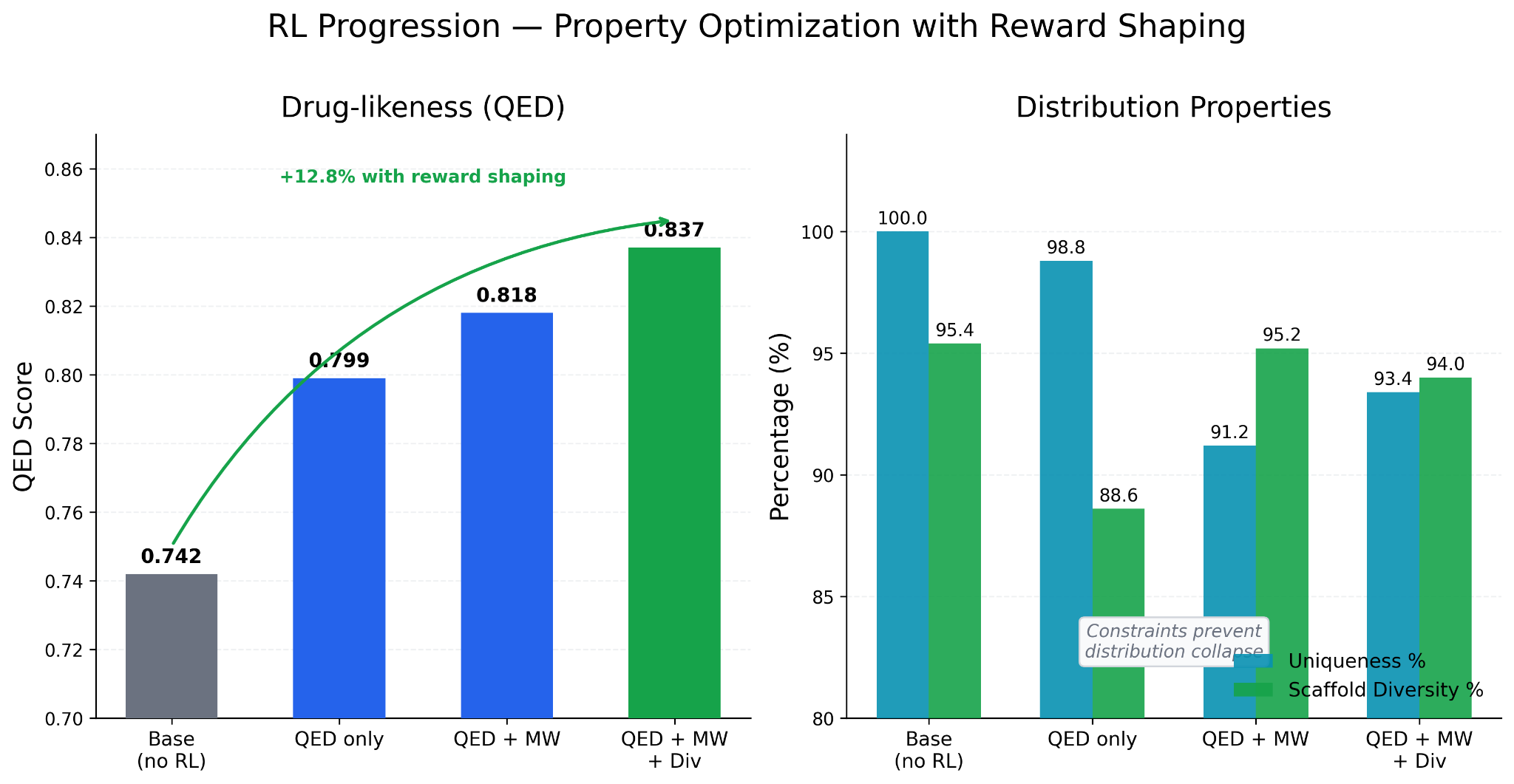
QED only: QED improved to 0.799, but the model concentrated property distributions into narrow bands. Scaffold diversity dropped from 95.4% to 88.6%. The model was finding higher-QED molecules by converging on a narrow region of chemical space.
QED + molecular weight: Adding an MW reward term broadened the distribution back out. Mean MW shifted toward 330 Daltons (closer to drug-like range), LogP distribution improved, scaffold diversity recovered to 95.2%. QED reached 0.818.
QED + MW + diversity penalty: Final QED 0.837, scaffold diversity 94%, uniqueness 93%. A 12.8% QED gain from baseline while maintaining structural variety.
Each constraint was added in response to a measured concern, not added speculatively.
Text conditioning
RL optimizes a single scalar. Real drug design needs richer control. We added text conditioning by extending the architecture with cross-attention layers connecting a frozen text encoder to the transformer backbone, plus a learnable MLP projector bridging the encoder output dimension to the transformer hidden dimension.
We trained on ChEBI-20, a public dataset of 26,000 molecule-description pairs, and used classifier-free guidance (CFG) at inference time: generate one candidate conditioned on the text prompt and one unconditional, then amplify the difference by a scale factor. We drop text conditioning with 10% probability during training to enable this.
Contrastive alignment
Before fine-tuning the diffusion model, we aligned text and molecule embedding spaces using CLIP-style contrastive learning (InfoNCE loss): pull together matched text-molecule pairs, push apart unmatched ones.
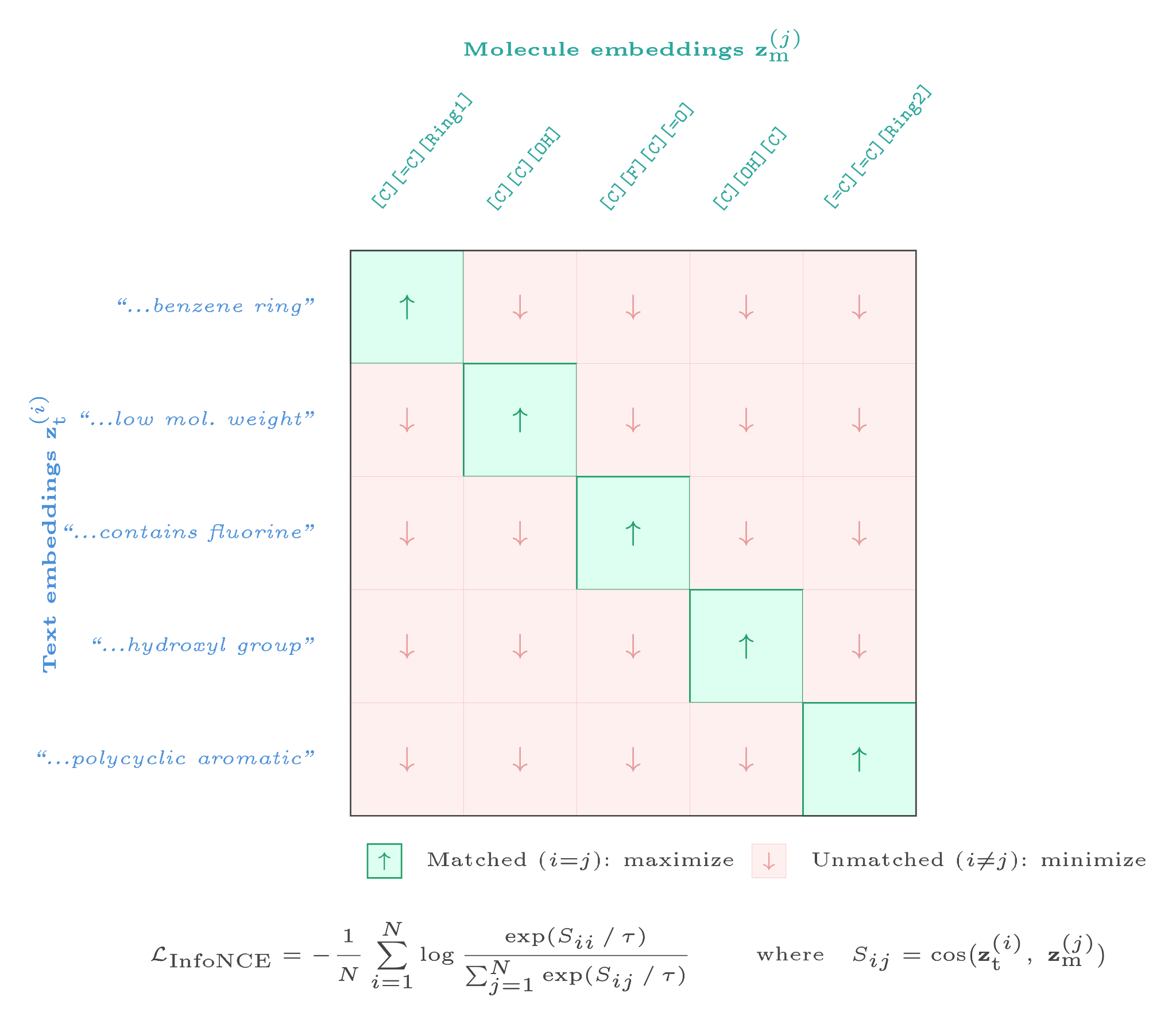
where $S_{ij}$ is the cosine similarity between text embedding $i$ and molecule embedding $j$. Pre-aligning the encoder to chemistry space before using it as a conditioning signal gave consistent improvements across all metrics.
Systematic ablation
Each step was motivated by the result of the previous one:
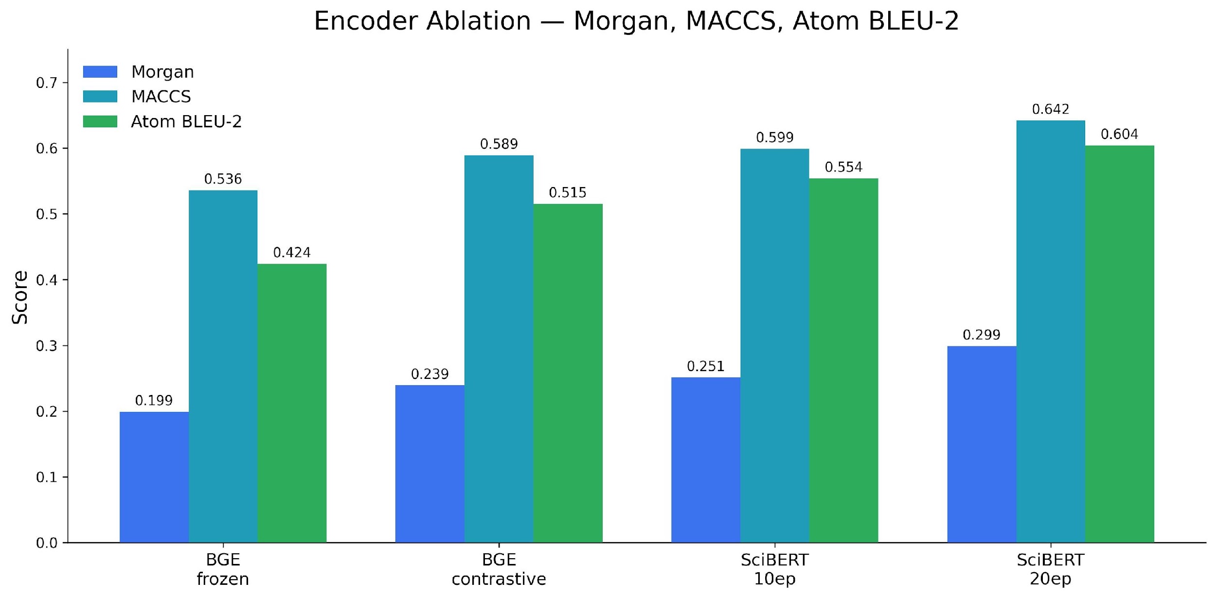
| Configuration | Morgan Tanimoto |
|---|---|
| BGE frozen (baseline) | 0.199 |
| BGE contrastive | 0.239 |
| SciBERT contrastive, 10 epochs | 0.251 |
| SciBERT contrastive, 20 epochs | 0.299 |
| + Inference reranking (N=10) | 0.310 |
BGE vs SciBERT: Swapping from BGE-large (1024-dim, general English) to SciBERT (768-dim, chemistry-pretrained) improved performance despite the smaller dimension. Domain-specific pretraining beat parameter count.
10 to 20 epochs: Validation loss was still decreasing at 10 epochs. Extending training produced the largest single-step improvement, 19%.
CFG scale sweep: We tested CFG scale from 0.5 to 3.0. Clean bell curve with peak at 1.5.
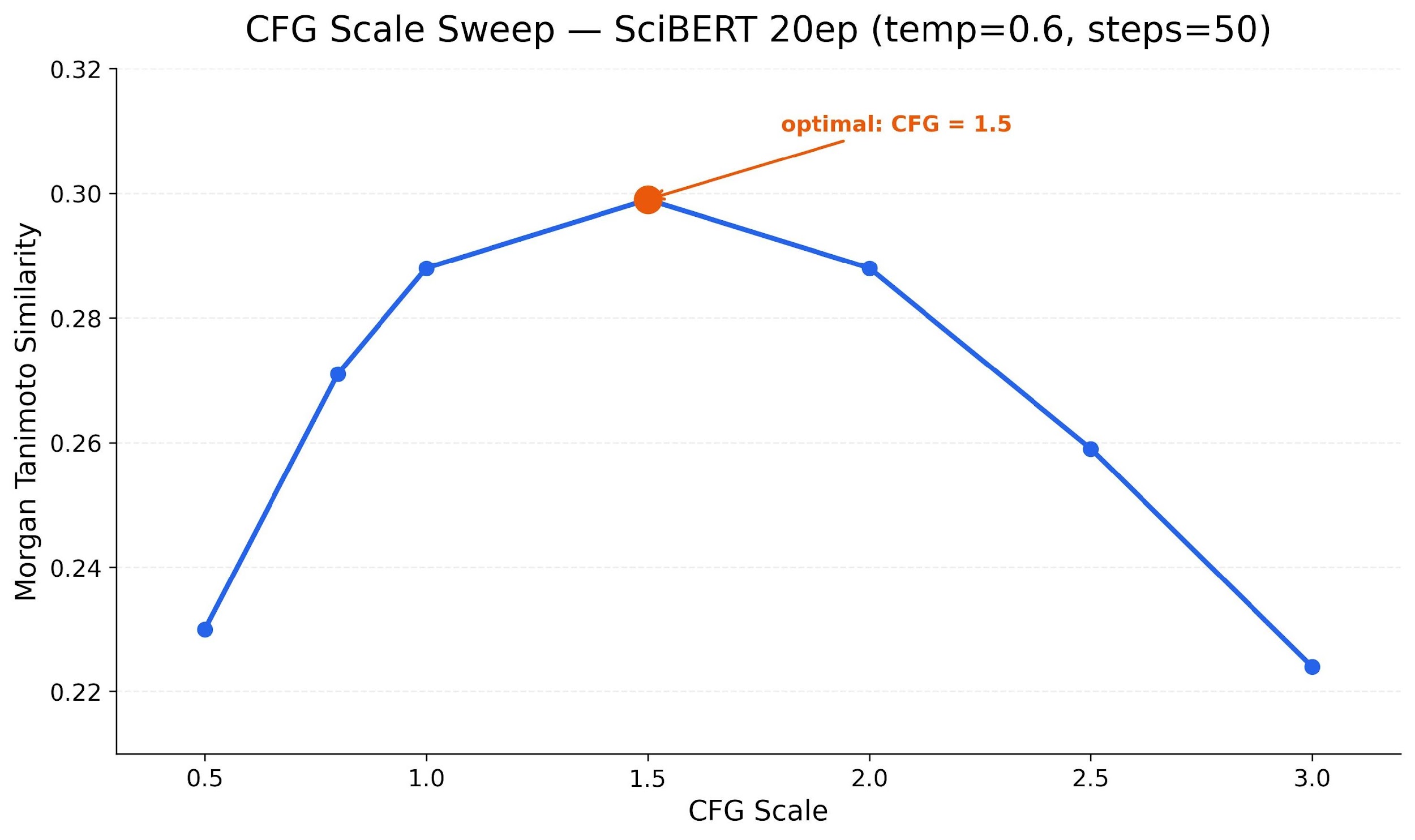
Too low ignores the text; too high collapses diversity. The same pattern as text-to-image diffusion.
Reranking: Generate 10 candidates per prompt, score with the contrastive encoder, keep the best. Small but free at inference time using the same model already trained.
Comparison against TGM-DLM
TGM-DLM (Gong et al., AAAI 2024) is a 180M parameter continuous embedding diffusion model — currently the strongest published method on ChEBI-20.
| Morpheus (27M) | TGM-DLM (180M) | |
|---|---|---|
| Morgan Tanimoto | 0.310 | 0.688 |
| RDK Tanimoto | 0.418 | 0.739 |
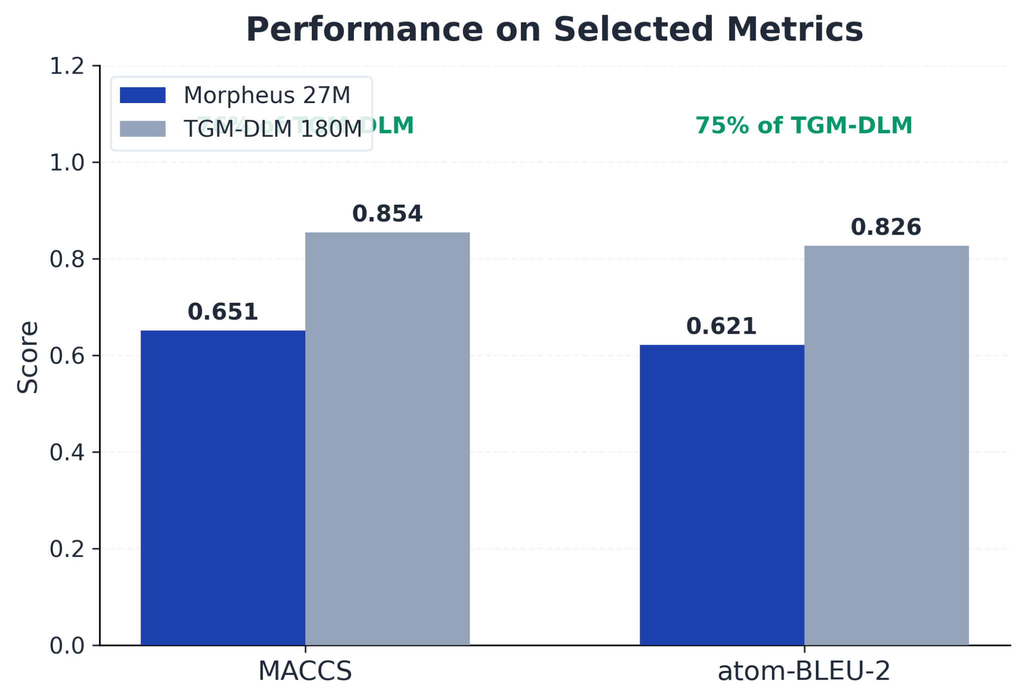
| MACCS Tanimoto | 0.651 | 0.854 |
| Atom BLEU-2 | 0.621 | 0.826 |
| Chemical validity | 100% | 87.1% |
| Hardware | MacBook M2 | A100 GPU |
76% of MACCS and 75% of BLEU-2 at 15% of the parameter count. On validity: TGM-DLM reaches 87.1% with a dedicated correction network. Without that correction it sits at 78.9%. We do not need a correction phase.
The Morgan gap (45% of theirs) reflects the ring topology failure measured directly in the next section.
Failure analysis: ring topology
The most useful result from the project is what we found when we stratified performance by molecular complexity.
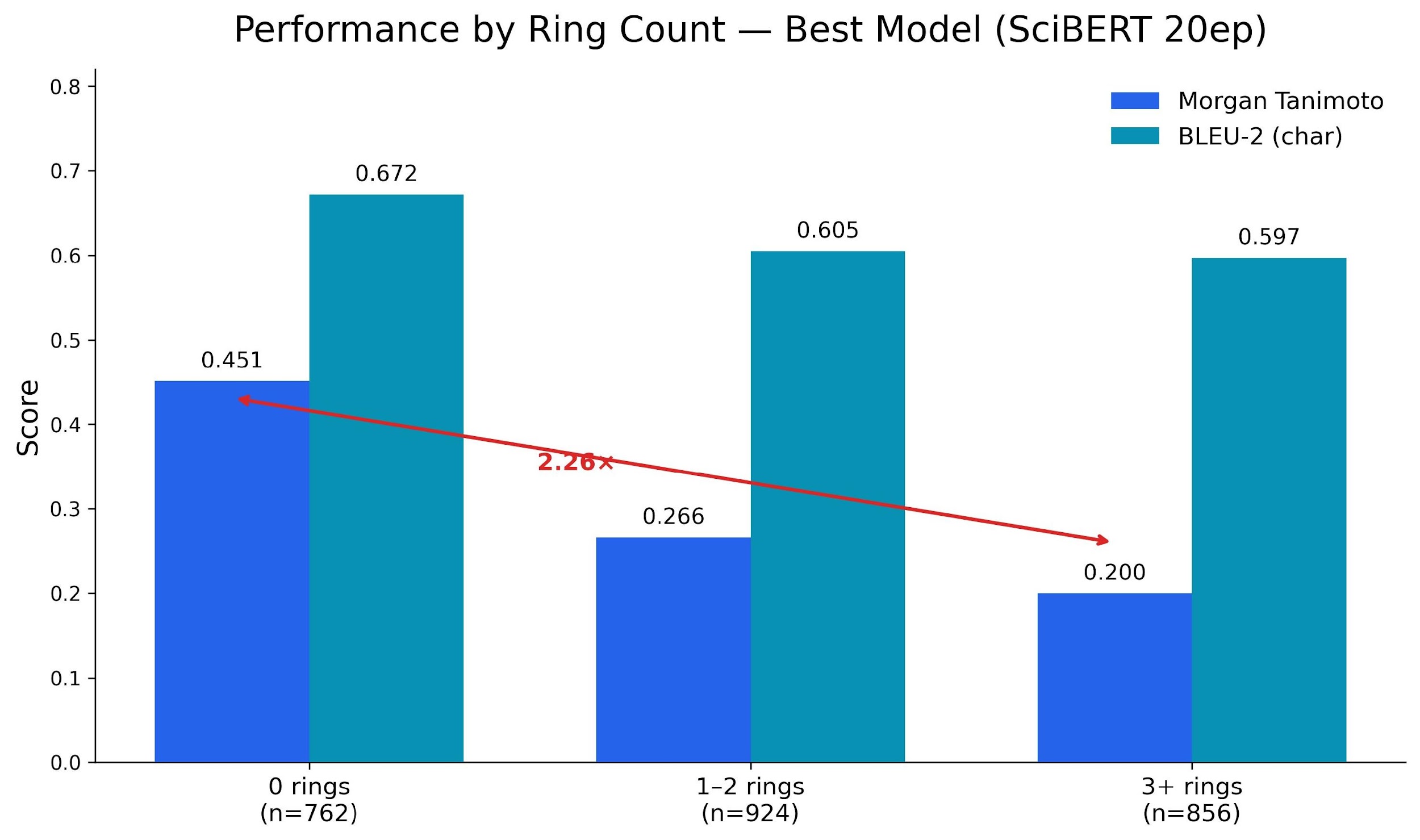
On acyclic molecules (chains, fatty acids), we reach Morgan 0.451. On molecules with 3+ rings, we drop to 0.200. A 2.26x gap. We traced it to the token level:
| Ring count | Ring count prediction accuracy |
|---|---|
| 0 rings | 96% |
| 1 ring | 57% |
| 2 rings | 44% |
| 3 rings | 32% |
| 5 rings | 17% |
| 6+ rings | 0% |
In SELFIES, ring closures use a count token that tells the decoder how many atoms back to bond with. Predicting that count correctly requires knowing which atoms appear in the intervening positions. In MaskGIT parallel decoding, those positions may still be masked when the count token is being predicted.
This is an architectural incompatibility between fully-parallel position prediction and closure tokens whose semantics depend on resolved nearby context. We ruled out implementation bugs through a five-check audit covering tokenizer integrity, truncation, round-trip verification, special tokens in count positions, and version consistency. All five checks clean.
We also documented three negative results: post-hoc EOS truncation hurts, iterative refinement adds nothing, and more denoising steps at inference time hurts. The interpretations of why are our best hypotheses, not directly measured.
The proposed fix is block diffusion: commit positions in groups so that count tokens see resolved context before being predicted. Not yet tested on molecular generation.
What we learned
Per-step RL gradients are necessary for diffusion. The naive single-pass proxy fails completely (QED collapses from 0.742 to 0.38). Per-step log-probability accumulation during the 50-step denoising process is necessary. Same principle as DDPO for continuous diffusion.
Modularity pays off. We swapped text encoders three times, added RL to the same backbone, and reused the contrastive encoder for both conditioning and inference-time reranking — without retraining the generator from scratch. The zero-initialization of cross-attention output projections is what enables this.
Representation sets the ceiling, not parameter count. At 27M we reach 75-76% of a 180M model on standard metrics. The remaining gap is discrete tokens vs. continuous embeddings, not model size.
Domain-specific encoders beat larger generic ones. SciBERT at 768 dimensions outperformed BGE-large at 1024 dimensions consistently across every metric.
What is next
Both RL and text conditioning work independently on the same backbone. The natural next step combines them: generate a molecule that scores high on a disease-specific activity classifier while satisfying a text description of its chemical properties.
For rings, block diffusion is the most principled intervention. We are also investigating whether the failure pattern holds at 150M scale, which would confirm it is representational rather than a capacity issue.
The 150M scaling study is still in progress.
Code available on GitHub.